Transformations and expressions provide the key to adapting STEM to a wide range
of applications. Can you explain the difference between calculations made in the
Editor and those performed at run-time? This technical article looks into the mechanics
of evaluating expressions and compares four classes of calculation in STEM.

Expressions in the STEM Model Editor
STEM allows you to create links between different inputs, and to calculate inputs
using algebraic expressions, just like you can in a spreadsheet. As a simple example,
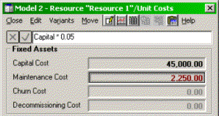
consider a Resource whose capital cost is known, but for which the maintenance cost
must be estimated at 5% of the capital cost. In the illustration below, you can
see that a simple formula is used to calculate this value, nicely illustrating both
the concept of an ‘internal reference’ and the use of a formula.
An internal reference is just a text label used to identify another input, analogous
to a cell reference in a spreadsheet. Rather than having to look up or remember
these labels, you can just click with the mouse while editing a formula to pick
up references to other inputs.
STEM automatically re-evaluates a formula whenever any of the ‘precedents’ (i.e.
the references made within the formula) are modified. This process is confined to
the Editor, and the calculated values are stored in the .DTM file when a model is
saved.
Time series
Expressions can also be used to relate and calculate time-series inputs. Whereas
the example above calculates just a single value, a formula entered for a time-series
input calculates a series of values for each year or period of the model run. For
example, if two complementary services are provided to the same customer base, then
you might define the penetration for the second service as:
- "Service 1".Penetration.RefValue
The resultant input is calculated for each period in turn, applying the same formula
to each of the corresponding values of the first input.
User Data
In addition to creating linkages between the standard STEM inputs, time-series expressions
can also be used to reference unbound User Data as user-defined inputs, providing
a completely flexible mechanism for extending the set of distinct inputs to a model.
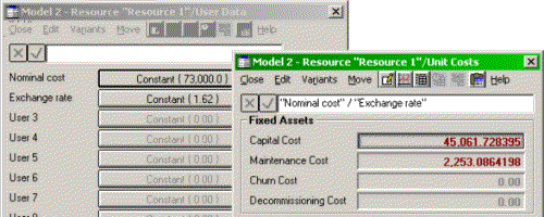
For example, for a piece of equipment imported from abroad, you might define User
1 and User 2 as Nominal cost and Exchange rate respectively (by selecting Rename
Field from the Edit menu in the User Data dialog), and then link these through to
the Capital Cost with a suitable formula, as shown below.
Linked defaults
Sometimes you may wish to share a common set of assumptions between several inputs.
For example, a set of lifetime data might be shared by several Resources, while
specifying different unit capacities. By selecting Defaults from the icon menu for
an element, you can identify a source element from which all unset values should
be inferred in the target element. Alternatively, and more intuitively, you can
use drag-and-drop to create this relationship directly. STEM captures this dependency
as a formula for the target element, which acts on each field in turn, except where
an explicit value has been entered.
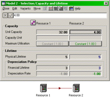
In the following illustration, the value entered for the Unit Capacity of Resource
2 overrides the default values linked from Resource 1.
External references
STEM provides comprehensive linkages with Excel and other database tools. Selecting
Links from the File menu in the Editor enables you to create an ‘external reference’
to scalar and time-series data from Excel spreadsheets, any ODBC-compliant database
or the inputs and results of a STEM model. The syntax for a link to Excel might
look like this:
‘C:\DATA[COSTS.XLS]Sheet3’!$A$2
which is the same format as is used in Excel for an inter-workbook link. The syntax
for linking to databases is described in detail in Section 5 of the User Guide.
Rather than create many parallel links between a STEM model and the same external
file, you can use the defaults mechanism to link several or all inputs for a given
element with one formula. This formula can reference a range of cells in a spreadsheet,
or rows in a database query, where the individual data are identified by labels
within the external file.

Run-time expressions and the STEM Model Engine
Transformations were first introduced in STEM 3.0 to satisfy a widespread desire
to model ‘equipment-driven demand’, that is to say a requirement for secondary equipment
to be dimensioned directly in terms of the installation of some primary equipment.
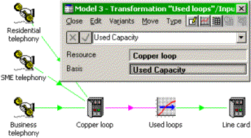
A simple example would be various services for differing customer segments requiring
a copper loop to an exchange, and then each copper loop requiring a line card at
the exchange. Mapping the demand directly from cooper loop to line card avoids the
need to repeat separate links from each service to the line card, as well as offering
a more intuitive representation of the actual network architecture.
A key attribute of a Transformation is that, within each period of the model run
cycle, STEM waits until it has calculated the demand for all the inputs of a Transformation
before calculating the Transformations own Output, and then proceeds to calculate
demand for any dependent elements. The ‘size’ of each input is defined by the input
Basis, in this example the demand for line cards being the number of loops actually
in use.
The simple Resource Transformation simply passes on demand, whereas, in general,
most Transformations actually modify their inputs.
Predefined Transformations
There are several ‘built-in’ Transformations for which the model engine performs
a standard parameterised calculation, as shown in the following table. Here the
Output of the Transformation is always calculated in the same way, but with the
influence of various input parameters, such as a multiplier, or a grade of service
for the Erlang B Transformation. These alternatives are accessed from the Type menu
in the Input and Transformation dialog.
|
Type
|
Parameters
|
Output
|
|
Multiplier
|
Time-series multiplier
|
A linear multiple of the input
|
|
Input–output mapping
|
Mapping, usually an interpolated look-up
|
A time-invariant non-linear mapping
|
|
Erlang B formula
|
Grade of service;sites
|
Number of circuits required (note: input is carried traffic, rather than offered
traffic
|
|
Time lag
|
Integer time lag
|
Input from earlier year
|
Expression Transformations
The most general Transformation element accepts a variable number of inputs (up
to 20 in STEM 6.2) and calculates its output from a user-defined expression. Although
this formula is entered in the Editor, it is not evaluated until run-time, as it
acts on intermediate results from the model engine, as identified by the bases of
the various Transformation inputs.
The canonical application is to sum a number of separate demands, such as two different
kinds of cards requiring slots on a shelf in a cabinet. In this case, Installed
Units is selected as the basis for both inputs, since this is what directly drives
space required on the shelf.
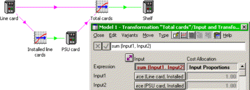
An Expression Transformation allocates costs in fixed proportions between its inputs
by default, but here the cost allocation basis is set to Input Proportions, prescribing
that costs should be allocated in proportion to the respective numbers of cards.
However, in this case, all costs will be ultimately fed back to the services driving
the line card.
The expression for such a Transformation is known as a ‘run-time’ expression, in
contrast to other expressions which are evaluated directly in the Editor. A run-time
expression may also include internal references to other inputs, so that for example
you can define additional parameters in User Data. However, it is important to understand
that, while User Data may be defined by a time-series formula or linked to Excel,
this is not possible for Transformation inputs, which serve only to identify intermediate
results for selected input elements.
The final technicality relates to copying run-time expressions. As far as the Editor
is concerned, a run-time expression is a value, so there is no distinction between
paste values and paste formulae for such a field. Moreover, if you link defaults
from one Expression Transformation to another, the form of the expression from the
first Transformation will be reproduced in the second. In contrast, a time-series
expression for the original User1 would yield only a set of default time-series
values for the second element.
Expression syntax for derived results
The STEM model engine is concerned with network business operations: the forecast
of demand and revenues, and the calculated incremental and total installation of
all types of equipment and other cost drivers. The investment required to fund this
business activity is calculated separately by an iterative process in the Results
program, with reference to the operational results from the model engine and certain
financial inputs from the Editor.
The reasons for this separation are twofold. Firstly, the calculations in the Results
program are done ‘on demand’, with no additional disk space requirements. (This
applies not just to the investment layer, but also to all intrinsic summations of
network revenues over Service elements and network costs over Resource elements.)
Nowadays, disk space is no great concern; the more persuasive factor is the flexibility
of the ‘derived results’ mechanism which delivers these financial results.
Derived results
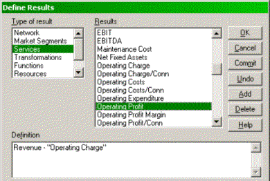
Select Define Results… from the Config menu in the Results program to explore this
feature for yourself. For each type of result, you will see a large number of pre-defined
derived results. For example, Service Operating Profit is defined as:
Revenue – "Operating
Charge"
This single definition applies consistently to all Service elements. The terms in
this expression relate to other Service results; when the result is calculated for
a given Service, the Results engine automatically addresses the respective results
for this element.
Network aggregation
Expressions for derived results can contain all the usual arithmetic operators and
algebraic functions. Special treatment is given to the sum() function. The conventional
use is to sum several other results, for example:
sum (a, b, c)
but if, for a network result, you write:
sum (Services.Revenue)
then this single-argument sum performs a sum of the given results over all the elements
of the given type. This method is used to evaluate all the network totals for revenue
and cost.
Collections
You can calculate automatic aggregations over arbitrary sets of elements by defining
Collections in the Editor. For example, if you select the two card Resources in
the example above and click the Collection button on the toolbar, the Editor will
create a Collection element, effectively grouping these two Resources. The Collection
provides a unified interface to the input assumptions for both Resources, and automatically
appears in the list of Elements in the Choose elements to draw dialog in the Results
program.
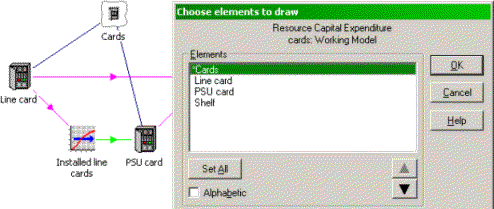
Derived network results may also refer to results for individual named elements,
most usefully for Collections, which can be used to provide a categorised breakdown
of costs versus revenues. ‘Defining results’ is explained in more detail in Section
4 of the User Guide.