STEM can be applied to almost any business topic and
always delivers a systematic and reliable treatment of time and money
within an intuitive and self-documenting visual metaphor.
 In our previous newsletter we sketched out the shape of a small start-up business as a teaser for an interactive modelling exercise over two days at the STEM User Group Meeting in September 2017. The intention was to explore three growth modes for Michaela’s Best Bread Direct service, from her first unconstrained vision, through a more sober and realistic measured phase and finally to a more ambitious, customer-driven approach.
1. Modelling reset
The inspiration for this exercise was the question: how would it work to start with a certain resource base and ‘see what you can do with it’, i.e., ‘sweat your assets’? Actually it is interesting to consider three distinct modes for a business plan:
- unconstrained: here are my revenues, here are my costs; do I have a business?
-
measured: how well am I utilising my assets; is this even realistic?
-
driven: link asset investment to forecast customer growth.
The latter is business as usual for STEM, but may not be where everyone starts. How straightforward are the simpler alternatives in STEM? We chose to explore these modes in an unfamiliar business context to avoid being stuck with ‘normal thinking’.
Michaela’s value proposition, initial customer segmentation and product portfolio are described in the earlier article. We will be more specific about the underlying assumptions in the sections that follow where the data are presented in the context of the calculations which they most directly influence.
An essential first step for her is to research or at least estimate the size of these segments within her target market:
- the likely buying patterns are a central revenue driver for a commodity business
- her initial penetration assumption is one big unknown and should be tied to expected yield of specific initial marketing campaigns
- another unknown is whether she can supply all of these customers single-handedly!!
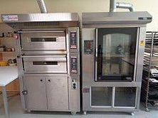
A few key pieces of equipment must be purchased upfront to make bread on a regular and ‘industrial’ basis. (These are persistent resources in STEM.) The majority of the day-to-day expenditure is for the ingredients for each of the offered products (which we will consider as consumable resources).
 As you will see below, Michaela has her numbers. It should be a breeze to see if she will make any money:
-
revenue = volume × price
-
cost = fixed + variable
The working hypothesis is that her mixer, oven and slicer will suffice. Our initial task is just to calculate the likely financial performance of the imagined enterprise.
2. Unconstrained: what I think we can achieve
Michaela intends to launch Best Bread Direct in the small town where she lives:
-
households = 3500
-
population = 8500.
Rather than look at the population in total, she segments the market by household type and estimates:
- the likely buying patterns for each
- pricing at ‘supermarket +25%’.
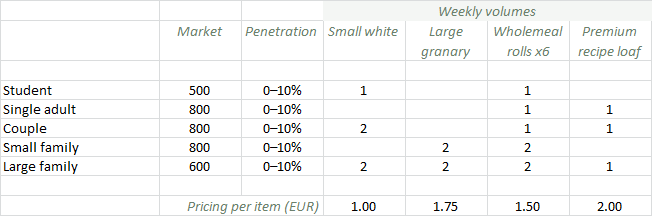
Figure 1: Demand and pricing assumptions
The actual customer numbers are hard to predict, but revenue is otherwise a reliable calculation as it is based on everyday consumption (which can be entered as an explicit weekly rate in STEM) and assured by cash or card at the point of sale. Revenue is also a direct output from a service in STEM, and so the first action is to create/populate the initial market and service elements. We need one market for each customer type, and then one service element for each customer-type × product combination so that we can capture all the distinct buying patterns. As you will see below, this is much easier than it sounds using the sublime copy and replace feature.
Note: STEM performs a native conversion of the weekly volumes above to an equivalent daily rate, independent of whether you generate results in months, quarters or years.
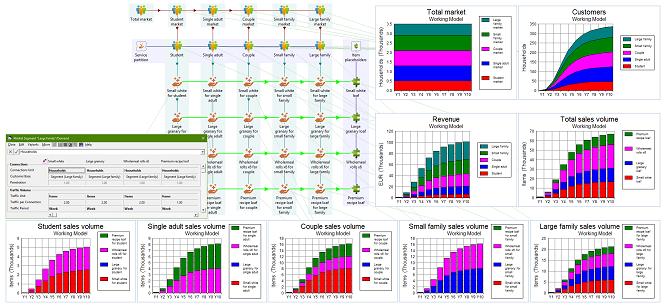
Figure 2: Market, customers, sales volume by product, and revenue
Note: we have added a column of placeholder resources for each of the products. Each provides a simple focus for aggregating the demand across different customer types and then serves as a consolidated driver for quantity-dependent production costs later.
Equipment costs are known (if the quantities are realistic). A naïve expectation would be to enter the unit costs into a number of separate persistent resources, and then ‘just get one of each’, but this is not ‘normal STEM thinking’! In the absence of an explicit driver for the required equipment capacities, we have to set the input Planned Units = 1.0 in order to ‘get one of each’ and thus be able to just ‘write down the costs’. However, we must consider exactly when the oven is required. To place the associated capex events in Y1, it is necessary to use an interpolated series for the Planned Units input in order to capture the intended timing more precisely (nothing in Y0, one unit in Y1).
Since the power consumption of the oven dwarfs that of the other equipment, and because the oven is likely to be left on for a fairly consistent baking period each day, this can be considered as a fixed cost in the initial analysis. The nominal power rating for each piece of equipment is scaled by the active proportion each day; i.e., the number of hours of operation as a proportion of 24.
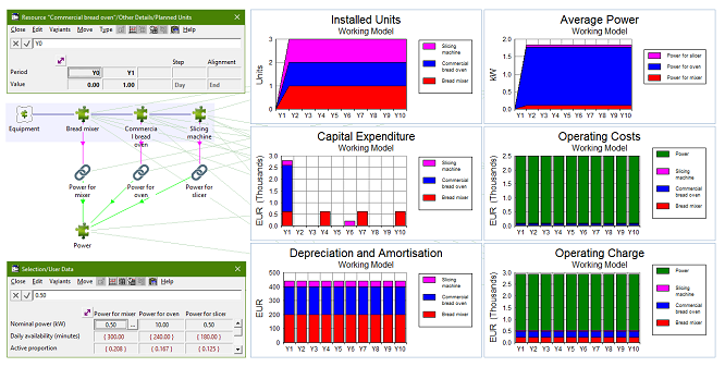
Figure 3: Fixed equipment costs and power
Our direct production costs are easy to project because they have either a per-customer or per-product-volume characteristic. We will use the recipes and unit costs illustrated in Figure 4 below to calculate the quantities and resultant total costs.
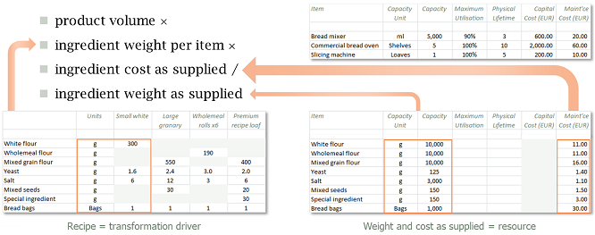
Figure 4: Direct ingredient costs scale with demand
The Consumption output of the per-product placeholder resources mentioned above is available as a driver for these calculations. Each ingredient will be a consumable resource and a transformation will be required to capture the relevant quantities for each product × ingredient combination.
It is tempting to write down all the products and required ingredients first, and then wire up the relevant combinations afterwards. However, this is likely to be a very repetitive task, with more or less the same structure and similar units needed for each combination. Generally it is much more efficient to work through one combination first, from end to end, and then use copy and replace to add further products and ingredients like rows and columns in a table, which adapts the relevant labels intelligently as it goes.
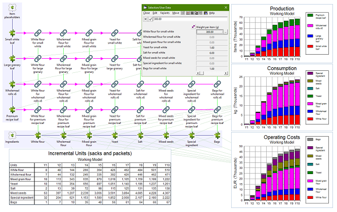
Figure 5: Recipes, ingredients and consumption
The financial results so far imagined are easy to generate. But are these results realistic:
- will the bread fit in the oven?
- are there enough hours in the day?
We will gain critical insights by attempting, however crudely, to measure the actual utilisation of the fixed assets. Each driver that we can add quantifies the load on individual resources, and can then be compared with actual performance, and thus used to validate the overall approach.
3. Measured: what I know we can achieve (and still have a life)
What are we missing? Besides practical issues like stock management and storage, there are no serious challenges with understanding direct costs. A business must obviously cover these costs in its pricing as the bare minimum to be profitable!
The more interesting questions relate to the dimensioning and utilisation of fixed assets. (This has been our principal focus historically, so one would hope so!) The essential reality check is whether the intended production is feasible with the planned asset base. In this second phase we will develop credible drivers for the main equipment (bread mixer, bread oven and slicing machine), as well as for the fuel required for deliveries and (most precious of all) Michaela’s time!
 A simple approach to estimating oven occupancy (or load) would be to look at the average daily volume and convert to required shelf-space. However, time is a critical element of the throughput capacity of any kind of food processor. If the oven is run ‘more than once’, then we must consider not just the space but also the time occupation of each product.
A key assumption will be for how many hours in the day the oven will be used. This will then enable a more authentic calculation structure based on, not just the required shelf-space per production item, but also for how long each item must be baked. Then the effective load of each item can be measured in sq m minutes as units of 2D-space × time.
We imagine that the daily schedule allows for some preparation time before baking, then the oven being on for perhaps four hours, and then further time for slicing afterwards. Each of these activities may overlap, but for logistical reasons each of them will be only a subset of overall production time, and all of this before making deliveries for as long as Michaela is doing this singlehandedly!
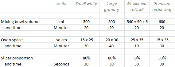
Figure 6: Production assumptions for mixing, baking and slicing
Note: we assume that items can be queued freely within the production cycle (i.e., everything must just be ready by the end of the overall baking period) so that we don’t have to worry about any kind of peak load as opposed to the simple average. For greater refinement we could consider daily variation from the norm, seasonal and weekend variations, or even seasonal promotions.
Just like the application of the recipes above, we must place a transformation for each product which captures the oven space-time required to bake one unit of that product.
A similar approach is used for the bread mixer where each product requires a certain quantity of dough which, in turn, requires an equivalent volume for a certain period in the mixer. Here the effective load of each item is measured in litre minutes as units of 3D-space × time. The transformations can be quickly replicated using copy and replace.
 The dimensioning for the slicing machine is simpler as it is driven only by a number of minutes per product, only for a subset of products (we don’t slice rolls), and only for a proportion of those actually sold (customer preference).
For now we defer the more usual STEM discipline of connecting these calculations to the resources themselves (which would tell you how many you need). Instead we first divide the total load for each activity by space capacity to calculate the number of minutes (i.e., time) required for each resource each day, and then divide by the length of the period available for each activity to calculate an effective equipment utilisation result. This needs to be < 100% in each case for Michaela’s vision to be credible!
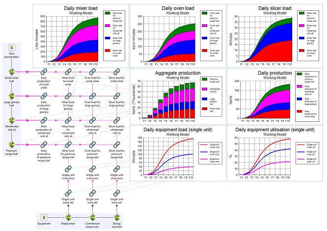
Figure 7: Equipment load and utilisation
We use the Trace Results command at each stage to check the results for plausibility.
Note: if everything is cooked at the same temperature, then we can simply aggregate the oven space-time for all products. Otherwise we must either ‘round up’ in ‘whole oven loads’ by product, or more pragmatically apply a Maximum Utilisation constraint (which is a standard resource input in STEM) to allow more generically for this kind of inefficiency. The same goes for the mixer where different doughs must be mixed separately.
 If Michaela’s (one) own vehicle will suffice, in terms of space/time, then all she may care about at the start is the fuel cost. Assuming there is room to spare, delivery costs will be a function of visits (customers), not volume, and of course ultimately distance and fuel.
Unless Michaela is lucky with proximity, she will probably need to traverse most roads to reach the first few customers, so we could use an explicit distance driver for the deliveries, regarding this as a separate value add (which could be readily outsourced too). However, it will be better still to capture this non-linear mapping from customer numbers to street distances so that the model has the dynamic built-in, and this is easy to achieve with the Input–Output Mapping transformation type in STEM.
Note: Michaela’s time will be more simply a linear function of visits. The driving time is only more significant when there are very few customers (when her time is less precious).
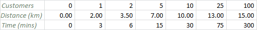
Figure 8: Delivery distances for increasing numbers of customers
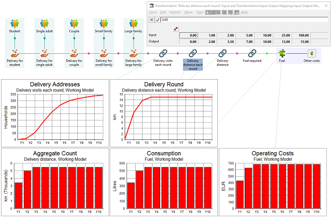
Figure 9: Deliveries and fuel
 Most business founders are guilty of not counting their own time! However, this is a precious resource, and it is also finite, especially if you want a life! Every task we have considered so far has a time cost (and there are plenty more besides), and this is all Michaela’s time in the early days. So it is essential to keep tabs on everything she has to do to see if her vision is actually feasible, and if she will ever sleep!
Our initial time estimates for these tasks are not differentiated by product, but the model is again structured with distinct inputs so they can be tweaked on an individual product basis once Michaela has the benefit of operational experience.
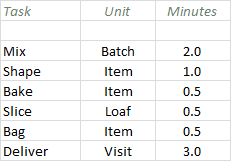
Figure 10: Time assumptions for production and delivery tasks (not including any admin!)
Note: for now we will assume that other tasks will keep her busy during ‘hands off’ time while dough rises.
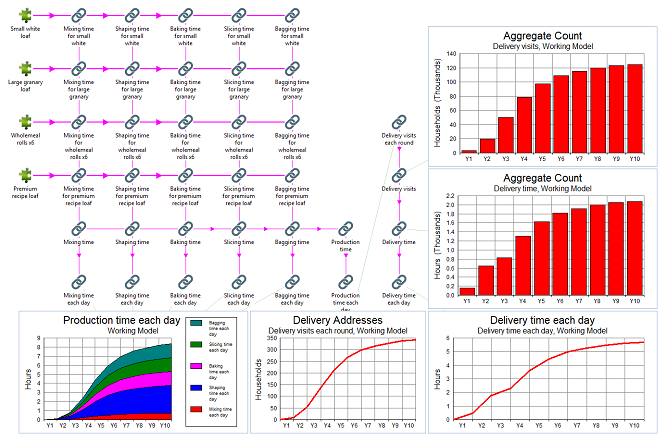
Figure 11: Staff time and utilisation
Michaela’s original intention to spend three minutes a day with each customer has to be reduced to one minute (on average) by Y3 otherwise she would need 17 hours a day just on deliveries. Fortunately her customers don’t have time to hang around chatting more than once in a while either!
Even then it is clear that, by the time she starts to achieve even her modest local growth targets, Michaela will no longer be able to run this business single-handedly!
The initial, driverless results may well indicate a profitable business if Michaela’s aspiration is good, but are these results actually achievable with the finite resources originally envisaged? We can use the built-in scenario manager in STEM to compare the results directly:
-
with drivers: the same revenue, but potentially increased costs (or alternatively, less revenue if consumption is limited by maximum output)
-
without: original costs, but potentially unachievable activity!
 We can explore more than one assessment of the drivers to provide a range of references to sanity check the original plan without necessarily abandoning it. We may regard this as a risk assessment for as long as the alternative stories don’t persuade us that the venture is flawed! With these more sober and measured approaches you can more credibly ask:
- is the business still profitable?
- will you run out of money?
- can you persuade someone to lend you the money for the oven?
- or even crowdsource it?
4. Driven: what do my customers want?
So far we have just looked at the ‘bare bones’ of the business, the things Michaela would need on day one just to make and deliver her first batch. In the longer term she will need to allow for various overheads and replacement tools when she decides it is no longer comfortable to rely on what there is in her domestic kitchen. Soon she will want some kind of basic accounting system and of course a marketing website in order to do the best she can in the immediate neighbourhood.
Family pressure may lead her to seek her own external premises, especially if she decides she wants to take on other staff, and she may need a dedicated vehicle if she wants someone else to do the driving. It’s not clear at this point if it will still be a viable business at this scale.
 However, she feels that many of these additional costs are out of proportion with the endeavour. You could do so much more with these assets; if only you could buy 10% of a van! With meaningful drivers for each resource we can compare the fully-loaded cost with the incremental cost per unit.
Michaela gets it: if you are going to be in business, then you need to reach a scale where your assets can be utilised efficiently. The fully-costed business is a fully-informed opportunity!
The Best Bread Direct business first came about, not just because Michaela loves bread-making, but because she believed there was significant demand for a quality product.
Rather than slam on the brakes when she worked out the previous numbers (after midnight again!), she saw what she must do:
- her business model was telling her that her current load was already
way past 100%, and that the trend was up
-
with a bigger team and more resources she could expand her market, increase
sales, and reasonably expect to find some efficiencies and economies of scale
- by plugging in some different scenarios for likely take-up and expansion costs (such as that van and industrial unit) she could forecast a best case and worst case with sufficient detail, rigour and flexibility to convince her savvy crowd-funders to invest in her growing dream.
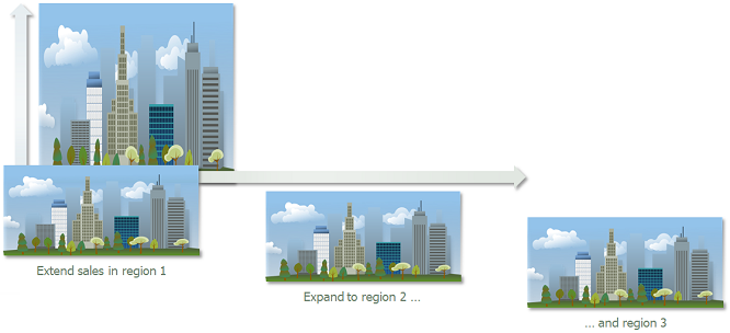
Figure 12: New sales targets, additional villages and other areas altogether with separate teams
There are numerous metrics you must watch as a business owner:
-
profitability: is the business actually generating value, month-on-month?
-
cashflow: is there enough cash at the bank to cover all the current outgoings?
-
interest cover: is the business rewarding you or your lenders?
-
net present value: would the cash be better invested elsewhere?
Each of these should be examined when comparing scenario results.
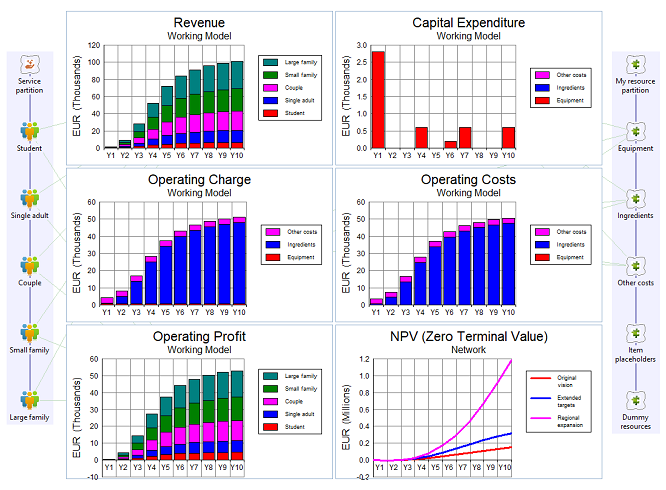
Figure 13: Financial metrics for the original model, plus extension/expansion scenarios for NPV
 Possibly the most critical decision Michaela will face is how fast to grow? Too fast could be scary, hard to manage, and risk crippling debt, but too slow might under-achieve on revenue, and be frustrating too! Michaela should flex her growth plans to span 2/3/4/5 years:
- four scenarios (parallel to the other dimensions already imagined)
- compare key performance and survivability metrics in the interim
- cumulative results over 5 years are the principal determinant, subject to criteria on the interim results.
 Running a business takes passion, confidence and endurance. Just when you feel like you have climbed one mountain, another summit looms in the distance. Building a business model demands focus and attention to detail, but also an instinct to ‘think the unthinkable’. Your model must be able to go with you into any corner, and still make sense to your audience.
The model outlined above is far from perfect. In fact it is little more than a beginning. Thinking through the more precise business realities and making corresponding tweaks to the model is where the fun starts. This article serves only to illustrate some of the issues you might consider if you are thinking about making bread for a living, and more generically how you could use STEM to create a robust and visual model of the financial dynamics of any start-up business.
Deconstruct your start-up
If you like the thinking in this article and would like our help to take your business apart in a similar way then please contact us. Our mission is to provide the tools and coaching to enable great minds to think more clearly about business logic in any sector and we will be pleased to assist you. You will not be disappointed!