Keeping a grip on complexity

STEM has a multi-dimensional scenario space for exploring key assumptions in a business model, plus the facility to automatically generate geographical variants of core model structures. In September 2005, we expect to demonstrate an integrated sensitivity analysis tool, as well as a system for fully re-useable model templates. In this technical article, we explore how these threads of complexity interact and how STEM can safely apply sensitivities to per-scenario instances of replicated model structures.

Creating scenarios is easy in STEM

Suppose you want to capture several different economic futures within a model, e.g. to explore the performance of different technology solutions, or to compare a colleague’s demand forecast with your own. We use a vastly simplified cellular model to illustrate these basic techniques, comprising busy-hour bandwidth requirements for 3G capacity across a number of base-station sites in a green-field network roll-out. In our base scenario, with roll-out over 300 sites over two years, increasing demand for higher bandwidth services quickly exceeds basic coverage capacity with standard carriers offering 2.5Mbit/s

Base scenario: busy-hour bandwidth and installed carriers

First we add an alternative technology solution which offers twice the bandwidth capacity in the basic carrier:

• Select Capacity and Lifetime from the Resource icon menu for the Carrier.
• Select the Unit Capacity field, and then select Create Scenarios… from the Variants menu. A new Variant Data table is displayed with three columns for Variants 1, 2 and 3, where the original value of 2.5 Mbit/s has been copied into the first row, which is identified with the Unit Capacity of the Carrier element.

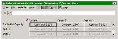
Original data copied into three variant colums

We rename the underlying Dimension element as ‘Technology’, Variants 1 and 2 as ‘Standard’ and ‘Enhanced’, and discard the third, unwanted Variant. The Variant Data for Enhanced is changed to 5.0 Mbit/s to reflect the higher capacity. We then move to the Capital Cost input, and repeat the process, this time electing to associate the new scenarios with the same Technology Dimension, which results in the original cost of EUR75 000 being copied into the second row. We set this to the higher cost of EUR125 000 for the Enhanced technology.

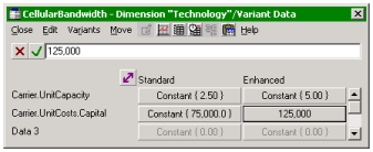
Scenarios named and calibrated

The two scenarios can immediately be run and the results compared, as shown below.

Enhanced technology promises reduced deployment and long-term capex

So far we have created scenarios for two related inputs which vary coherently. Now we compare two different demand forecasts by choosing a new Dimension when creating scenarios for the Penetration and Nominal Bandwidth per Connection inputs. We rename this Dimension as ‘Demand’, with Variants ‘My forecast’ and ‘Alternative forecast’, and then enter alternative demand data in a separate variant Data table.

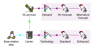
Two-dimensional scenario space

This approach allows these demand parameters to be varied independently of the technology, resulting in four distinct but consistent scenarios which can be examined in parallel. As the following picture shows, the Enhanced Technology pays off in the long term with the Alternative forecast, but not with the original demand parameters.

Enhanced Technology pays off only with the Alternative forecast

Geographical variants are defined in a similar way

The economics of cellular networks are better in urban areas, where cell utilisation is greater and backhaul is cheaper. We add geographical variants to our model in order to capture these effects as follows.

• First select the icons, 3G services, Base-station sites and Carrier, and then click the Template button on the toolbar in the STEM Model Editor. A new Template is created, referring to these elements, and which we rename as ‘Geo-type’.
• Click the Variant button on the toolbar to create four related Variants, which we rename as ‘Metropolitan’, ‘Urban’, ‘Suburban’ and ‘Rural’.

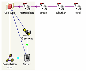
Template structure

The key distinctions to capture are the split of subscribers, and the number of sites required to provide coverage for each geo-type. Typically the subscriber base is weighted towards the urban centres, while the rural areas require the greatest numbers of base stations.

Split of subscribers and number of sites required for each geo-type

As with scenarios, we create variants for these parameters, but in this case, the Variant Data are associated with the Geo-type Template, and the differing values are applied to four copies of the original elements within the same, expanded model.

Replicated model structure

Separate but consistent calculations are thus made for resource utilisation, capex and revenue for each geo-type, and then aggregated for the network as a whole.

Per geo-type and aggregate results

Adding scenarios for individual geographical variants

So far we have looked at scenarios and templates in isolation. Suppose we want to combine both techniques? This is fine if a scenario parameter is completely separate from any Template, and in fact presents no problem if the scenario parameter is within the scope of a Template, provided that it is invariant with respect to replication (i.e. is not a Template parameter). The two examples above can happily co-exist because the scenario Variant Data for Unit Capacity and Capital Cost for the Carrier, and Penetration for 3G services, will be first copied into the master Template, before being copied identically to all replicas in parallel with the separate Template Variant Data for Customer Base and Sites.

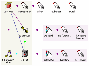
Independent scenario and template variant data

However, if in the original Template we added scenarios directly for the number of subscribers, then these data would be overwritten when the Template was replicated and each separate geo-type customised with the Template Variant Data. In order to preserve the scenario data, it is necessary to create scenarios for each of the Template Variant Data, i.e. one row in the scenario Variant Data for each column in the Template Variant Data.

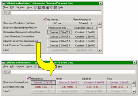
Scenario Variant Data for each column in the Template Variant Data

We are developing functionality to automate this process such that when you ask to create scenarios for a field which is already a Template parameter, STEM will automatically create scenarios for each of the Template Variant Data associated with that field.

The process of exploring sensitivities

A business model is only ever as good as the assumptions behind it, and when there are very many inputs, it can be hard to know which of these merits the most careful research. Therefore a key part of the modelling process is to perform sensitivity analysis, i.e. to determine the relative impact of various model assumptions on the main outputs. Although this can be done manually with the existing scenario management functionality, we are making this easier with the introduction of dedicated sensitivity elements which will automatically generate consistent results sets for a model (‘deltas’) where one or more parameters are perturbed by plus or minus a number of percentage points (or absolute steps, or steps between explicit minimum and maximum values).

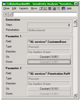
Sensitivity analysis parameters

The STEM Editor will allow you to create multiple, overlapping sensitivity sets, and to choose which (if any of these) should be run with the existing selection of scenarios to run. The Results program will automatically select the appropriate delta results sets for graphs when you ask to graph a given sensitivity – you won’t have to worry about how many steps are generated.

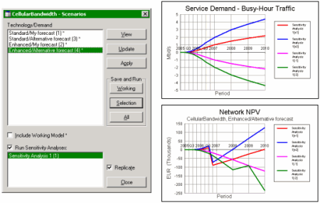
Sensitivity analysis results

In addition to the simple charting of comparative time-series results, i.e. all delta results sets shown on one graph as shown above, we will also provide options to create so-called tornado charts which highlight the relative sensitivity of separate, independent inputs.

Keeping it all together

In this article we have considered scenarios, geographical variants and sensitivities. In order to make effective use of these three techniques, and especially when combined in the same model, it is essential sooner or later to understand how the underlying mechanisms interact. Fortunately there is a simple, fixed sequence as follows:

The good news is that sensitivities can be directly superimposed on any combination of scenario parameters. However, sensitivities for Template parameters must be applied to the corresponding Template Variant Data, as per scenarios.

Note: if you want to explore sensitivities with explicit minimum and maximum values, it may be necessary to create scenarios for these values if they are to be applied to scenario variant data. We aim to consider all possible eventualities!

My account (log-in)

© Implied Logic Limited

Contact | Downloads | Core team and advisory board