At least 50% of a service provider’s costs relate to operations and maintenance,
as opposed to basic capital expenditure. Sadly, many business models are left with
rough estimates for these aspects – often estimated as a rule-of-thumb percentage
of the capital cost – rather than being modelled explicitly via any kind of task
analysis.
In fact, the STEM resource concept is just as readily used to capture activity costs,
such as spares or staff costs, as it is to represent capital costs. There are just
some areas where care has to be taken when mixing absolute and incremental quantities,
and when switching between annual and quarterly results.
This article illustrates some of these points through a series of examples which
may serve to stimulate existing thinking on the topic, and also offer specific techniques
for those actively involved in this kind of modelling. It also highlights
one specific area of confusion, and suggests a potential solution which could be
added into STEM to round out this capability.
Using task estimates and resources to forecast headcount
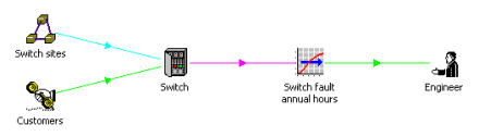
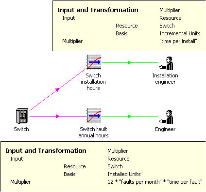
Consider a Switch resource which requires regular maintenance to attend to recurring
faults or typical unplanned incidents. Since this is driven from the total
installed base, this is relatively easy to model, using two basic ingredients:
- a transformation combines user data assumptions for the annual rate of fault incidence
and the average number of hours required to correct a fault, to calculate an annual
fault hours result (which you can think of as an instantaneous annual rate)
- an Engineer resource derives its capacity (as a matching instantaneous annual rate)
from user data assumptions for weeks per year, hours per week and effective utilisation.
Matching estimated task hours to engineer capacity
This approach works fine, even in a quarterly context, because only a quarter of
the salary cost is charged each quarter. An increasing salary can be modelled
with a cost trend; and a learning curve effect could be modelled within the Average
Correction Hours per Fault input, factoring in a floor and (decreasing) multiplier.
The engineer may also be shared by different types of equipment.
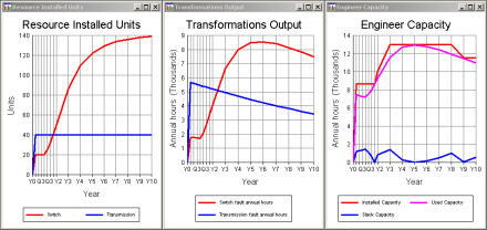
Annual task hours and required engineer capacity
An engineer working 48 × 37.5 hours a year, at a utilisation of 80%, could
result in some of the 1440 annual hours being left slack. Alternatively, if
the engineer is shared from a company pool, then you could use a lower hours-per-week
assumption to define a lower capacity. Or, if the engineer is sub-contracted,
it might be more appropriate to define the costs as an operations cost that would
only arise from actual usage, even if the hourly rate might be higher for this kind
of ‘pay as you go’ approach.
The traditional flaw of this kind of modelling approach is its direct sensitivity
to the fault rate assumption, but scenarios may be used to estimate best and worst-case
requirements.
Adding dependent staff and support assets
The standard technique of using a transformation with a basis of resource installed
units can be used to model a variety of dependencies from the engineer, such as
administrative support, manager and vehicle resources, each of which may be characterised
with a capacity measured in (supported) engineers. In a more complicated model,
these secondary support resources might be shared by different types of engineer,
or the engineer resource might be shared by different types of equipment. Some of these resources may need to be separately based at more than one physical
location, readily modelled with the usual STEM deployment concept.
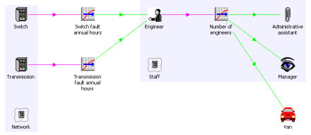
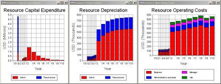
Secondary support resources and opex breakdown
Handling short-term contracts
One potential issue, which arises if demand is falling, is that a STEM resource
has a defined lifetime (currently not less than one year), and so you may end up
with an engineering cost for a few quarters after a switch is no longer required. The same issue would apply to customer support staff resources if demand was falling
each quarter.
One obvious fix for this would be to allow a lifetime less than one year – though
it is not clear how this would work in a model running in years. But it might
be preferable to be able to say that a resource could be a ‘transient asset’ which
would disappear as soon as it is not required (perhaps equivalent to setting Redundant
Unit Decomm. Prop. = 1), or better still, to have a release time which could capture
notice-period effects.
Another approach would be to think of the capacity of a resource in terms of an
absolute number of tasks that need to be done in a period, and for such a resource
to only ever exist within one period (of whatever size). This idea is explored
in more detail below in the more general context of incremental effects.
Quantifying installation engineer time in an annual model
So far we have been looking at activities related to total demand or installation,
as these can be readily matched to an instantaneous annual effort rate. If we constrain our attention to models running exclusively in years, then it is
also straightforward to model equipment installation rates and required manpower
levels, again in two stages:
- incremental units of the same Switch resource can be scaled by hours per installation
to calculate the annual hours required, which can be used as the capacity of an
installation engineer
- an Engineer resource derives its capacity (as a matching instantaneous annual
rate) from user data assumptions for weeks per year, hours per week and effective
utilisation (just as above).
Installation-rate and annual fault-rate transformations
But the implicit assumption that the incremental units can be matched to annual
capacity falls to pieces in a quarterly or monthly context, as we shall see in the
following examples.
Interpretation issues for incremental quantities in a quarterly or monthly model
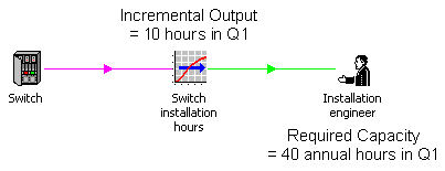
Consider two cases: one unit installed in each quarter versus four units all installed
in Q1. In the first case, if we want to match to a resource with a capacity
specified as an annual rate, we would need to scale up by factor of four in a quarter
to get the same share of a permanent resource; i.e., to say that we need 40 hours
in a year if we are to have 10 hours in each quarter. (Bear in mind that only
a quarter of the salary is charged each quarter.) This can be achieved by
using the periodLen() function in a formula for the multiplier.
In a case where all the incremental units are in the first quarter, then this would
be fine if the resource capacity did not persist beyond the quarter. It makes
sense that 40 hours would be required in that quarter: potentially more staff are
being employed on a shorter contract.
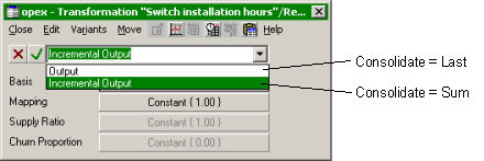
But how should the Output result be consolidated (i.e., presented in annual format
when a model has been run in quarters or months)? In general, it is assumed
to be instantaneous (as per most demands in STEM), and so we take the value from
the final period in a year; but this would completely hide the transient in the
case of everything being installed in Q1. So STEM is currently coded to accumulate
an incremental units basis during a year specifically to avoid this problem.
But then this leads to too much capacity of the resource being required in later
quarters, if the periodLen() approach is used to scale up the demand in Q1.
Alternative representations of quarterly incremental demand
A potential solution for comment
Suppose instead that we were to introduce an aggregate-mode transformation (or output),
which would not cumulate over the year, and which would be consolidated by summation. This would not be able to use the periodLen() approach, as the output for a quarter
should relate only to the increment in that quarter (and would be summed across
quarters on consolidation), but STEM could understand that the periodLen() scaling
should be built in when matching such an aggregate demand to instantaneous capacity
of a resource. That is, the demand (derived from incremental units) would be
10 hours in the quarter, and this would turn into a requirement for 40 hours per
year instantaneous capacity of a resource. (Or we could also introduce an
aggregate-mode resource whose costs would be associated with aggregate demand in
the current period only, and not scaled as a proportion of a year – this is
the concept of a ‘transient’ resource mentioned above.)
Matching incremental output to annual capacity required
For the Results program to know how to consolidate such an output, we could have
two types of transformation; or, more manageably (and with much more general clarity),
we could add a second, Incremental Output basis for transformation outputs. So you would choose which basis was being used when linking from a transformation.
Transformation output bases and related consolidation modes
For single input transformations, you could infer the mode from its input; whereas
an expression transformation would have to specify the user’s intention. The
resource Incremental Units basis would be an aggregate input, as would service traffic
(volume) and revenue (as opposed to the currently scaled Annual Traffic and Annual
Revenue bases).
Either the ‘other’ mode would be left at zero; or perhaps more usefully, a standard
output could be cumulated from incremental output within a year as per the current
incremental units basis, and an aggregate mode could be inferred as a delta of two
consecutive periods? This needs more thought.
However, separating these two outputs and classifying them properly would enable
STEM to make more meaningful and reliable calculations which would make sense in
both annual and quarterly contexts, and more generally any combination of periods
which might be required.