If you have already used the Elements tab for selecting
results to graph in STEM 7.5, then you may be familiar with:
- the Variants tab, which appears if you use template
replication
- the Cost Breakdown tab, which appears when cost-allocation
results are available by resource.
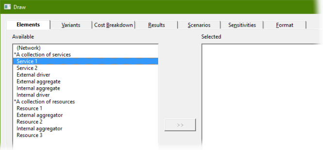
Figure 1: The full set of tabs which may appear in the Draw
dialog, depending on model structure
This technical article explains how the interface for drawing graphs has been streamlined
in STEM 7.5 with dimensional (i.e., orthogonal) selection of elements, variants
and contributing resources by default, and more specific Linear
Selection of individual combinations when required. We illustrate how
even a dimensional selection may result in a sparsely-populated graph, and consider
the complexities of notation and selection when cost-breakdown results are required
in a model in which services and/or resources are replicated from a template.
Dimensional selection vs linear selection
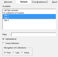 The Variants tab is a big improvement on earlier
versions of STEM where all variants of a given element would appear in the same,
flat list of elements as all variants of every other replicated element, as well
as every other non-replicated element! The new interface in STEM 7.5 allows you
(by default) to select the relevant variants independently from the original element
names (dimensional selection). This complication
is suppressed altogether if you are not using replication, or if you have not selected
any elements to draw which are replicated themselves (left–right filtering between
tabs). You can also select any defined collections of variants in this tab in the
same way that you can select collections of regular elements in the initial Elements tab.
The Variants tab is a big improvement on earlier
versions of STEM where all variants of a given element would appear in the same,
flat list of elements as all variants of every other replicated element, as well
as every other non-replicated element! The new interface in STEM 7.5 allows you
(by default) to select the relevant variants independently from the original element
names (dimensional selection). This complication
is suppressed altogether if you are not using replication, or if you have not selected
any elements to draw which are replicated themselves (left–right filtering between
tabs). You can also select any defined collections of variants in this tab in the
same way that you can select collections of regular elements in the initial Elements tab.
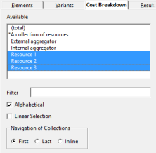 The Cost Breakdown tab provides a similar dimensional
approach for selecting contributing resources when drawing allocated-cost results
for services or transformations. By default, you can select the resources (RHS)
independently from the services (LHS), much as you could with the original 2D Selection in earlier versions of STEM. This complexity
is also suppressed if you are not using cost breakdown, or if you have not selected
any elements to draw for which cost-breakdown results are available. Again, you
can also select any defined collections of contributing resources in this tab.
The Cost Breakdown tab provides a similar dimensional
approach for selecting contributing resources when drawing allocated-cost results
for services or transformations. By default, you can select the resources (RHS)
independently from the services (LHS), much as you could with the original 2D Selection in earlier versions of STEM. This complexity
is also suppressed if you are not using cost breakdown, or if you have not selected
any elements to draw for which cost-breakdown results are available. Again, you
can also select any defined collections of contributing resources in this tab.
With this default dimensional approach, STEM graphs all of the available combinations
of the items selected in each tab most generally as a ‘full cube’ of
services × variants × resources. The logic has been switched round so
that now you can check the Linear Selection option
in either tab in order to choose potentially a sparse subset from a flat list of
all the available (filtered) combinations. (Previously you would uncheck
2D Selection to the same end.)
It gets complicated if you explore cost breakdown results in a model which also
uses replication, and this was inelegant in earlier versions of STEM which had no
dimensional support for template variants. How this works, with and without Linear Selection in STEM 7.5, is explained in the
remainder of this article.
The more common case where a template is self-contained
When you learn about replication, your first templates are likely to be
self-contained in the sense that there is no dependency or cost-allocation
between one template instance and another. Consequently the only meaningful allocations
to an individual instance of a replicated service, such as
Service 1 / Variant 1, will be from resources, either outside of the
template altogether, or within the same template instance, such as
Resource 1 / Variant 1. For as long as this hypothesis is valid, it suffices
to write Service 1 / Variant 1 / Resource 1 for
this contribution (or just S1 / V1 / R1 for short
in this article). We will consider the more general case below.
In each of the Variants and
Cost Breakdown tabs, no selection (or checking the
Disregard Selection option) indicates ‘no detail required’.
In dimensional mode, each tab includes a special item which enables you to combine
the total with the detail on the same graph:
- an (all variants) item in the
Variants tab indicates the sum over all variants, and
- a (total) item in the Cost Breakdown
tab represents the plain (total) service result.
When the selections are dimensional, STEM graphs all the available contributions
based on the selected services, variants and resources. The special all/total labels
will appear within the legend of a graph to differentiate these items from the more
specific variant or breakdown items, but not in the minor title when no such detail
is included.
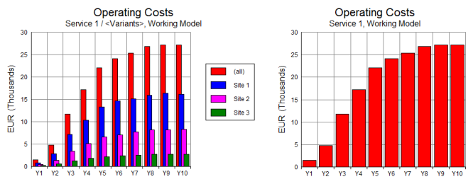
Figure 2: Distinguishing (all) from individual variants
in a legend, but not for a whole graph
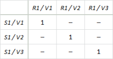
The resulting graph may be intrinsically sparse
if:
- one service is replicated and another isn’t, or is replicated by a different
template, in which case not all of the possible service/variant combinations will
exist
- not every combination of the selected services and resource is actually connected
- if you use the Format tab to hide zero-values or
unavailable series; or
- if you subsequently remove such series altogether with the
Remove Series command.
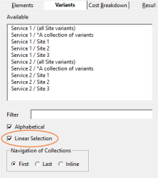 When Linear Selection is checked in the Variants tab, then S1 / (all variants)
appears in the Available list before
S1 / V1 and any other variants, and then the same for every other service
selected in the Elements tab. When
Linear Selection is checked in the Cost Breakdown
tab, then S1 / V1 / (total) appears in the
Available list before S1 / V1 / R1 and any
other resources, and then the same for every other service/variant combination selected
in the Variants tab. These options enable you to
choose a sparse subset of the available combinations directly.
When Linear Selection is checked in the Variants tab, then S1 / (all variants)
appears in the Available list before
S1 / V1 and any other variants, and then the same for every other service
selected in the Elements tab. When
Linear Selection is checked in the Cost Breakdown
tab, then S1 / V1 / (total) appears in the
Available list before S1 / V1 / R1 and any
other resources, and then the same for every other service/variant combination selected
in the Variants tab. These options enable you to
choose a sparse subset of the available combinations directly.
The new option to slice a selection for a graph
(so that only one item from a dropdown short-list is shown at any one time) can
be used for elements, variants or cost breakdown in dimensional mode. If you apply
this to filter an existing graph with sparseness, then STEM will re-instate any
series that it needs in order to display the same number of series for each slice.
If the original graph was intrinsically sparse, then some series will be shown as
N/A in any slice where there is no data (such as a non-replicated element when sliced
by variant). This could even apply to every series on a graph if you made a suitably
arcane selection!
When service and resource variants don’t match
 If a model exhibits only the kind of intra-variant or covariant allocations
described above, then the specific combination, S1 / V1 / R1 / V1,
will always yield the same results as S1 / V1 / R1 / (all variants)
because R1 / V1 is the only resource variant which
contributes to S1 / V1. There is no need to specify
the resource variant names as the label S1 / V1 / R1 is
already understood to be shorthand for S1 / V1 / R1 / (all),
the results for which always match those of S1 / V1 / R1 / V1
in these circumstances.
If a model exhibits only the kind of intra-variant or covariant allocations
described above, then the specific combination, S1 / V1 / R1 / V1,
will always yield the same results as S1 / V1 / R1 / (all variants)
because R1 / V1 is the only resource variant which
contributes to S1 / V1. There is no need to specify
the resource variant names as the label S1 / V1 / R1 is
already understood to be shorthand for S1 / V1 / R1 / (all),
the results for which always match those of S1 / V1 / R1 / V1
in these circumstances.
In the more general case, both ‘sides’ of a service/resource pair must
be qualified by the relevant variant; e.g., S1 / V1 / R11 / V11.
This distinction is only apparent when Linear Selection
is checked in the Cost Breakdown tab, and even
then the extra RHS variant detail is only shown if a selected service/variant combination
and related resource exhibit inter-variant allocation; i.e.,
at least one contribution from one variant to another. So it would be
possible to see the following items in the same list of Available
combinations:
- S1 / V1 / R1 exclusively covariant
allocations to S1
- S1 / V1 / R2
- S1 / V2 / R1
- S1 / V2 / R2
- S2 / V1 / R11 / (all variants) inter-variant
allocations to S2
- S2 / V1 / R11 / V11
- S2 / V1 / R11 / V12
- S2 / V1 / R12 / (all variants)
- S2 / V1 / R12 / V11
- S2 / V1 / R12 / V12
Note: you can see that the various contributions line up best if the initial sub-string
of the service (LHS) variant is always shown. We have shown that, if the allocation
is covariant, then S1 / V1 / R1 is actually equivalent to S1 / V1 / R1 / V1 (and
also S1 / R1 / V1 for the same reason), but suppressing the second variant provides
the most consistent experience when combined with the fully-qualified names for
inter-variant allocation.
This kind of inter-variant allocation can arise if one replicated element ‘drives
another’ via an intermediate aggregator resource. This technique is most commonly
used to link two separate templates, but our recent showcase model illustrating
The IT value-chain in a data
centre actually uses it to link two separate calculations within the same
template.
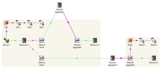
Figure 3: Inter-variant allocation from resources in the same template or a separate
template
In this more general case, even if you select (filter by) only one variant of a
given service, there may be resource contributions from other variants in the same
template, or from another template altogether which might not have been relevant
to the original element selection (and hence not shown in the
Variants tab). Rather than implement a secondary Resource
Variants tab just for this specific (and fairly obscure) case, the
current behaviour is that:
- all of the secondary variants (and (all)) are included
on a graph by default, or
- they can be selected individually (as illustrated above) if you opt for Linear Selection in the Cost Breakdown
tab.
Not the thing to worry about mid-project
This is not functionality that came about overnight! The original vision of making
everything filtered and ‘dimensional’ did not entirely prescribe how
things should work when a spare subset is required for a graph, or when there is
inter-variant allocation.
In the original draft design, we had the Variants
tab ahead of the Cost Breakdown tab (as it is in
the production system), partly because replication is the more commonly used functionality,
but more fundamentally because conceptually you need to choose a service variant
before determining which resource contributions (and variants) are relevant to it.
In subsequent design iterations:
- we briefly considered switching this around so that the
Variants selection could be applied equally to LHS services and RHS resources
- whereas the compelling factor is that the variants should be filtered as soon as
possible to limit the (potentially huge) number of cost-breakdown pairs offered
- if anything, a secondary Resource Variants tab might
be useful, but it is a toss-up between ‘ease of use’ and ‘too
many controls’ at this level
- the original design is reflected in and appears to be borne out by the pragmatic
choice of labels which show the LHS variant rather than the RHS variant in the most
detailed Linear Selection view in the more common
case of covariant allocation.
Some of the presentational details we have outlined here only became apparent after
we had a functionally almost-complete system to test, and so it was a prolonged
exercise to wrap this all up with a consistent and satisfactory experience for the
user.
As you might expect, collections of elements which are replicated translate into
being members of collections by individual site and by collective region when a
model is replicated. There is great flexibility to combine manual grouping by collection
with systematic aggregation by template, and thus to determine costs allocated to
one specific group of services from another specific group of resources at any level
without writing any hard-to-maintain formulae. STEM is the go-to
application for understanding cost allocation and controlling organisational spending
at scale.
What is entirely new (and miraculous by comparison with older versions of STEM)
is that all of these selections can be modified in situ
for an existing graph if you don’t get it right the first time or, more commonly,
need to add elements to an existing graph later.
STEM users can be thankful that they don’t have to do any
of this in a spreadsheet!
Note: every result described in this article, including the most complicated inter-variant
allocations, can be exported to Excel. Every graph selection (even with slicing)
can be published faithfully and reliably online with an Enterprise STEM (eSTEM)
server licence.