Managing a leaky reservoir

As a ‘wake-up exercise’ on day two of the recent STEM User Group Meeting, we explored a classic ‘leaky bucket’ problem of water supply, concerning a huge filling reservoir (HFR).

Creating a simulation of the varying water level in the reservoir over an annual rainfall cycle required a careful distinction between instantaneous and aggregate transformation outputs and some manual intervention to classify correctly the output mode of one or two key Expression transformations.

The potential addition of new Previous, Accumulation and Delta transformation types may facilitate a more natural expression of the logic which would remove the ambiguity about classification.

1. Managing water supply through the buffer of a reservoir

Consider a reservoir of maximum capacity = 5 million m³ (or cu m). (This is only 1km × 500m × 10m.) Imagine monthly rainfall varying between 4–20cm (subject to seasonal variation) over a collection area of 50 km² (sq km), of which 50% trickles through into the reservoir feeder channels.

If we estimate the downstream supply rate for an average (subject to differently phased seasonal variation) of 100 litres per customer per day for 1m subscribers, then how ‘bursty’ can the weather be without either:

• the reservoir overflowing, or
• the reservoir drying up (and the downstream supply with it)?

1.1 Care when defining the traffic for a service

It is tempting to try setting up a service with an area of rainfall collection as the ‘connection’:

• Connections = 50 sq km
• Penetration = 50%
• Traffic per Connection = x cm

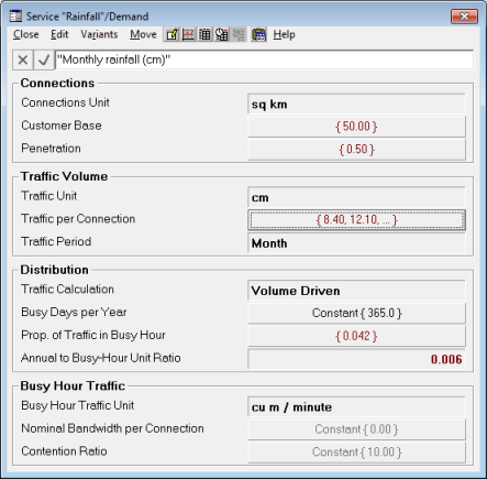
Figure 1: Rainfall per unit area is not the same as traffic per connection

However, this is not ideal as the Traffic result output would be measured in cm and the required 1000 × 1000 / 100 unit conversion would have to be factored in a separate transformation.

The traffic volume input should be entered in actual traffic units per (‘dimensionless’) connection.

We should work with monthly rain volume from the start, and we shall proceed with:

• Connections = 1 Catchment
• Penetration = 1.0
• Traffic per Connection =
  Collection area (sq km) × 1e6 ×
  Monthly rainfall (cm) / 100 ×
  Retention proportion

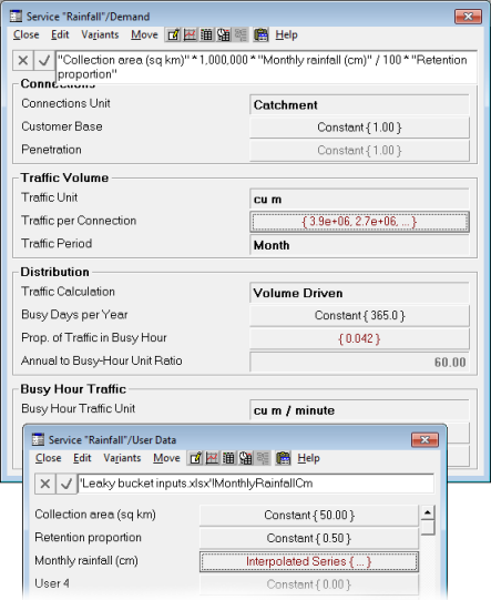
Figure 2: Working with monthly rain volume from the start

The traffic distribution reduces to flow in the (non-biased) busy hour. So we need to divide by 60 to measure Busy Hour Traffic in cu m / minute.

1.2 Flow in and out of the reservoir

Consider for the reservoir, each month, the flow of water in, f_i, and the flow of water out, f_o. We can simulate the ongoing volume of water (or water level) in the reservoir, vol , in terms of:

• its capacity, cap = 5,000,000 cu m
• the flow down of rainfall from the catchment area, f_d
• the flow required by customers, f_r
• the volume at the end of the previous period, vol’.

It is not hard to write out the following difference equations:

• vol = vol’ + f_i – f_o
• vol’ = prev (vol)
• f_i = min (f_d, cap – vol’ + f_o)
  limited either by actual rainfall or remaining available capacity
• f_o = min (f_r, vol’ + f_i)
  limited either by actual customer demand or current water level

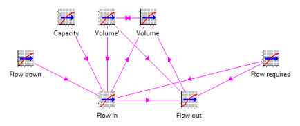
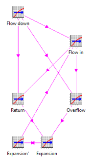
Figure 3: Graphical representation of the dynamical system

1.3 Removing the inherent circularity

From the equations and associated commentary, it is clear that there is a mutual dependency:

• the flow out may be limited by the flow in if the water level is low
• the flow in may be limited by the flow out if the water level is high.

But only one limit applies, depending on whether there is more or less rain than demand. So a closed solution exists in both cases and these can be reconciled with a conditional expression:

• if there is less rain than demand, then all the rain can flow in
• if there is more rain than demand, then all the demand is satisfied.

This allows for a convenient substitution in either case:

• if ( f_d < f_r)
• f_i = f_d
• f_o = min (f_r, vol’ + f_d)
  substituting f_d for f_i
• else (f_d ≥ f_r)
• f_o = f_r
• f_i = min (f_d, cap – vol’ + f_r)
  substituting f_r for f_o.

So we can write:

• f_i = if (f_d < f_r, f_d, min (f_d, cap – vol’ + f_r) )
• f_o = if (f_d ≥ f_r, f_r, min (f_r, vol’ + f_d) )

As the circularity is already removed, we can leave f_o more economically as-is:

• f_o = min ( f_r , vol’ + f_i )

1.4 Aggregate and instantaneous transformations

Even though the units throughout are cu m, the flows are aggregate (in period) while Volume and Volume’ are instantaneous measures. (See the proceedings of the STEM User Group Meeting for a similar example of relative and absolute distances for a mountain bike, all measured in km.)

However, there are no reliable clues in the formulation of the respective transformations: so far everything ‘looks aggregate’ to STEM (at least by default). So we have to ‘help’ classify Volume as instantaneous (in order to get the correct consolidation of results). The classification is inherited by Volume’, and then we have to also override the ensuing warnings for the subsequently mixed inputs to Flow in and Flow out.

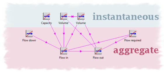
Figure 4: Contrasting output modes

Please contact Implied Logic Support if you need help with similar issues in your own models.

1.5 Limitation and unsuitability of the Time Lag transformation

This model (and specifically the link from Volume to Volume’ ) would be fine running in years; but the Time Lag transformation does not support a sub-annual lag, and even if it did, what you really want is the immediately previous period, regardless of its length.

As a temporary workaround, the model described here uses a specially modified copy of STEM which allows an input of Time Lag = –1 and which it understands to signify that it should return the value of its Volume input from the immediately previous period, regardless of whether the model is running in months, quarters or years:

• vol’ = prev (vol )

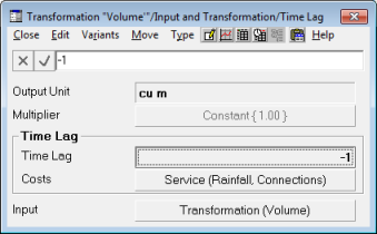
Figure 5: Using a specially modified Time Lag transformation pending the addition of a Previous type

It is clear that a new Previous transformation type would be useful for such aggregate models. Like the Time Lag, it would require a separate Costs input to avoid any circular cost allocation structures, but there is no obvious requirement for it to support more than ‘one step back’.

1.6 What comes in must go out

To avoid warnings at run-time, our final transformation(s) must drive a resource to ‘sink’ the demand. We assume a capacity of 1 cu m per minute (using an implicit time factor).

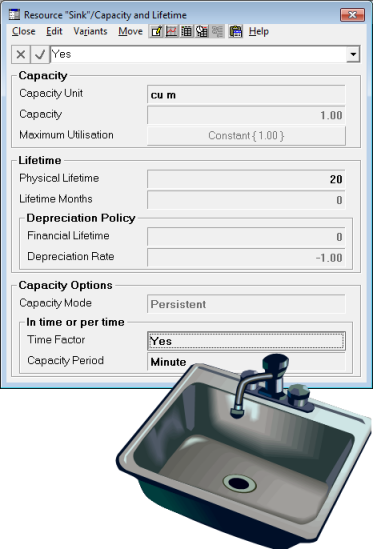
Figure 6: Defining persistent resource capacity with an implicit time factor to match a flow rate

Of course STEM will under-estimate the number of Sink resources required if their capacity is assumed to be fully utilised (i.e., water draining all day long)! In order to install a valid number of Sink resources, we would need to define a suitable Deployment:

• Sites = Customers.Size
• Distribution = Extended Monte Carlo

2. Metering the incidence of overflow

Based on its assumptions of seasonally varying rainfall (most in February) and consumption (most in August), with a randomised slant to the rainfall, the model calculates monthly results for the various flows modelled and the actual water level.

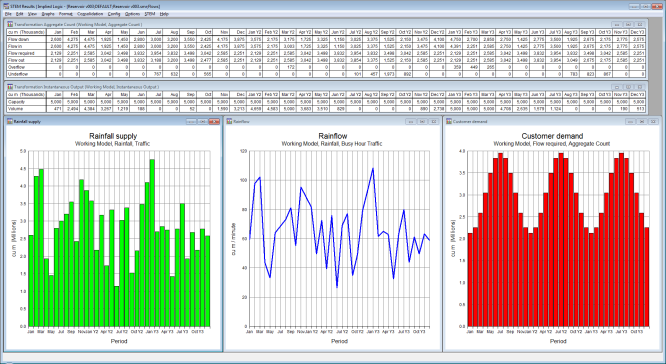
Figure 7: Seasonal rainfall (unpredictable) and customer demand

We can further monitor the Overflow = f_d – f_i and Underflow = f_r – f_o to meter how much water is lost and does not transition through the system in the winter, and to what extent the reservoir cannot meet the demand from customers in the summer.

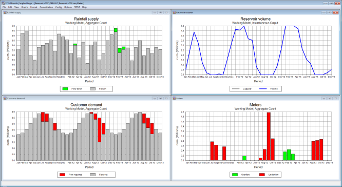
Figure 8: Reservoir level, rainfall overflow and demand underflow

3. Allowing for an expansion chamber

An alternative formulation of the classic ‘leaky bucket’ algorithm adds an expansion tank to the system. Excess rainfall is stored (queued) upstream from the reservoir and then passed through the system during a later lull (analogous to ‘traffic shaping’ in a communications system). In order to structure this extended problem, we consider:

• the volume of water in the expansion chamber, exp
• any flow presented to the reservoir later, return
• the volume at the end of the previous period, exp’.

Thus we can write (with modifications shown thus):

• f_i = min (f_d + exp’, cap – vol’ + f_o)
  modified to allow for any return from the expansion chamber
• f_i = if (f_d + exp’ < f_r, f_d + exp’, min (f_d + exp’, cap – vol’ + f_r) )
  ditto for the conditional version
• overflow = max (0, f_d – f_i)
  now possible for f_i to exceed f_d
• return = max (0, f_i – f_d)
• exp = exp’ + overflow – return
• exp’ = prev (exp)

Then you can see in the updated results the rainfall overflow, expansion, return and thus reduced underflow (to end customers at the summer peak). The overflow in Jan–Mar is returned in the subsequent lull of Apr–May. The expansion chamber fills, and then empties when the overflow is over. The next underflow or shortfall is mitigated by the return from expansion.

The Overflow variable now meters how much water is queued to transition through the system later.

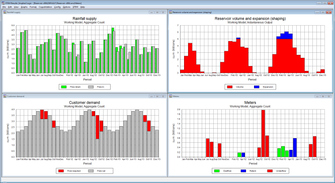
Figure 9: Rainfall overflow, expansion, return and reduced underflow

Compare this with the results if the expansion facility is disabled. Overflow in Jan–Mar is not returned in the subsequent lull of Apr–May. So the next underflow or shortfall is worse for loss of return from the expansion chamber.

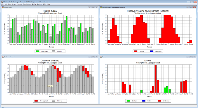
Figure 10: Corresponding results if expansion is disabled

4. Addressing the issues about classification of output mode

Working through the logic so far required manual intervention in two places:

• to signal to STEM that the Volume transformation should be aggregate, and
• to override the warning about mixed inputs to the Flow in / out transformations.

These issues suggest two further new transformations, in addition to the Previous type already mentioned.

4.1 Encapsulating and classifying an accumulation function

The Volume transformation uses a reference to Volume’ to calculate a cumulative value, vol = vol’ + f_i – f_o, and we have used the same approach for Expansion. This result could be achieved more elegantly using the prevThis() function, vol = prevThis (0) + f_i – f_o.

This would remove the circularity (and the ‘clashing’ links both ways) and also allows for the definition of the initial volume in the reservoir. The ‘previous’ element, Volume’, need only be added if required for other calculations (as it is here).

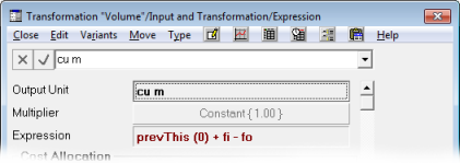
Figure 11: Using the prevThis() function to make an implicit reference to the previous value

Better still would be to have a new, purpose-designed Accumulation transformation type (strictly, an accumulation over time) which would avoid requiring specialist knowledge of the prevThis() function. It would also need an Initial Value input, like the prevThis() function it would replace, but crucially it would be designed to expect an aggregate input and make its output instantaneous, thus obviating the need for one manual intervention.

Note: the ‘previous’ element would be obsolete if an alternative Previous Output basis were available when selected as a transformation input. However, this was frowned upon at the recent STEM User Group Meeting where the consensus was that such an approach would obfuscate the logic compared to the greater visibility of an explicit Previous transformation.

4.2 Recognising a delta when you see one

The Accumulation idea also suggests a converse Delta transformation type which would expect an instantaneous input and make the output aggregate, defined as input – input’.

However, this would not have helped classify the more complex expression for f_i :

• f_i = if ( f_d + exp’ < f_r , f_d + exp’ , min ( f_d + exp’ , cap – vol’ + f_r ) )
  with its instantaneous / aggregate inputs.

The strict rule in STEM 7.3 is that the inputs considered by an expression transformation must all match on output mode (either instantaneous or aggregate). Once we override this constraint for f_i, STEM then correctly determines this must be aggregate as at least one of the inputs is aggregate.

The new transformation types suggested above would address the most common cases where STEM can’t determine the output mode automatically, and then the ‘aggregate if any input aggregate’ rule might be sufficient in all other cases.

5. Summary and applications more relevant to telecoms

With only minor modifications, we have a leaky reservoir model which generates realistic results for both Meter and Queue modes:

• the addition of a Previous transformation
• manually classifying the Volume transformation as instantaneous
• relaxing the strict consistency checking of inputs for f_i .

Leaky bucket algorithms like this are commonplace in the design of traffic management for packet-switched networks, although evidently a much shorter sampling period would be required to model this aspect of an ATM switch in STEM!

Another more relevant and credible telecoms example would be a queue of incoming customer requests for service activation:

• f_d would represent requests
• f_r would represent fulfilment.

My account (log-in)

© Implied Logic Limited

Contact | Downloads | Core team and advisory board