A client recently enquired as to whether STEM could be used to relate customer demand
on a call centre to underlying server costs according to varying service-level targets
such as, ‘the probability of a wait in excess of 5 seconds should not exceed
10%’.
 The objective is to be able to dimension the underlying system of resources to achieve
a target maximum probability for the wait in a
M/M/k queue to exceed a certain
wait threshold. For a given arrival rate, service time and postulated
Halfin-Whitt delay function, P(y),
how to find the value of y which satisfies prob (wait >
threshold) = target, from which
the number of servers required can then be inferred?
The objective is to be able to dimension the underlying system of resources to achieve
a target maximum probability for the wait in a
M/M/k queue to exceed a certain
wait threshold. For a given arrival rate, service time and postulated
Halfin-Whitt delay function, P(y),
how to find the value of y which satisfies prob (wait >
threshold) = target, from which
the number of servers required can then be inferred?
Note: conceptually the wait threshold described
above represents the limit of acceptable performance and such a
target probability would be referred to as a blocking
probability in the context of the Erlang B formula
analysis more familiar to current STEM users. The waiting probability arising from
the Halfin-Whitt delay function is actually very
similar to that given by the Erlang C formula.
1. A typical goal-seek problem
There are many references to the underlying mathematical analysis in the literature,
but the specific query was whether there was any way that a user could embed the
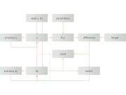
required goal-seek algorithm into a STEM model. If you generalise the structure
of this problem as follows, with f(y) representing
the combination of the delay function and the subsequent probability calculation,
then the real question is how would you get STEM to calculate
y?
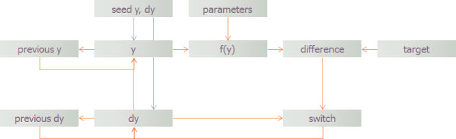
Figure 1: Generic structure of a goal-seek problem
The idea is to seed the y and
dy variable with appropriate values, such as 0 and 0.1 respectively,
and then calculate the current value of f(y). According
to whether this is below or above the target (i.e.,
a positive or negative difference) then set dy
to be the same as before if still below the target, otherwise set
dy = –previous dy / 2 in order
to home-in on the target. Then set y =
previous y + dy and continue …
which looks a lot like the prescription for a macro script!
2. Iteration in the Editor
One of the lesser known and more infrequently used capabilities of the STEM Editor
is its ability to use controlled iteration to resolve convergent calculations based
on circular references between a set of input fields in a model. A simple example
would be:
- User 1 = User 2
/ 2
- User 2 = User 1
+ 1
Such a construct is not much use by itself, but becomes interesting if other parameters
feed into the loop (e.g., set User 2 =
User 1 + User 3 above), and can be the
only way to resolve certain arithmetical systems where no closed form exists for
the solution.
With a healthy dose of confidence and only a modicum of care, it is not so difficult
to capture the parameters and terms of the Halfin-Whitt delay
function above within a series of User Data
in a STEM model. If you manually seed y = 0 and
dy = 0.1, and then replace first
dy and then y with the appropriate formulae,
STEM will then iterate through the formulae as desired so as to home in on the required
value of y, and then calculate the required number
of servers.
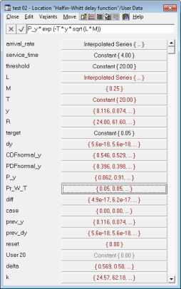
Figure 2: Using iteration to find a convergent solution for circular references
in the STEM Editor
With a degree in ingenuity from a well-known UK university, it is possible to extend
the simulation to include a reset variable which
will detect a change in the input parameters and force an automatic re-seed of dy and y so that
y can be re-calculated automatically after changing
any of the input parameters.
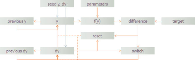
Figure 3: Goal-seek problem with automatic reset to seed new calculation
Since the User Data are all time-series variables,
it is actually possible to generate a graph of the output by making any of the inputs
(including the target probability) vary in time,
so you can get a direct understanding of the impact of changing the service level.
Note: the alert reader may have noticed that a standard simulation of the ‘error
function’, erf(), was slipped into the final STEM
7.3 release at the last minute. It was required as part of the formulation of the
Halfin-Whitt delay function in order to implement
f(y). So if you fancy a challenge, there is nothing
to stop you implementing your own version of this function once you have downloaded
and installed STEM 7.3!
3. A new Goal Seek transformation
This is all very well if all the parameters are known in advance in the STEM Editor,
but the calculation will be much more usefully applied to a dynamic quantity such
as the output of a transformation calculated at run-time. In fact the support for
aggregate measures in STEM 7.3 lends itself very well to this kind of problem where
you might want to calculate and work with the actual volume of call-centre events
in a given period.
So the obvious next step is to look to implement a new type of
Goal Seek transformation in STEM which would encapsulate an equivalent
iterative logic as described above and with the general structure outlined in Figure 3. An important detail to understand is that,
while this transformation will benefit from multiple dynamic inputs plus static
user data just like the current Expression transformation,
the planned iteration will be limited to the internal calculation of the output
of that transformation. It will continue to be the case that
circular references between separate transformations are not allowed.
In fact, the Goal Seek transformation will have
a lot in common with the Expression transformation, including the
Cost Allocation factors to weight individual inputs, but its output will
not be defined directly by the expression. For each period of a model run, the transformation
will iterate a search variable, y, to achieve a
given target for a user-defined function (the expression) of (i) its inputs, (ii)
any static user data and (iii) the search variable, and instead the transformation’s
output will be y.
According to our draft specification, and compared to the current interface for
an Expression transformation, the Goal Seek transformation
will require the following additional parameters:
- Target Value as time series,
default = 0.0
- Seed Output as time series,
default = 0.0
- Seed Increment as time series,
default = 1.0
- Refine Factor as double,
default = 0.5
- Maximum Iterations as integer,
default = 100
- Tolerance as double,
default = 1.0e–09.
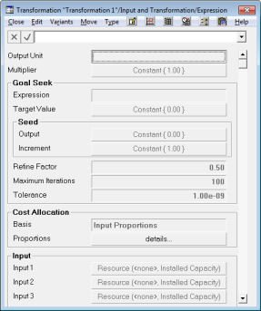
Figure 4: Mock-up of the dialog interface for a Goal Seek transformation
It is clear that by no means all expressions will be amenable to a goal-seek strategy.
The expression must at the very least reference the output variable,
y, and ideally it will be a monotonic function with respect to y;
though that may not be essential so long as the seed values are well chosen. A run-time
error will be raised if the output fails to converge to within the desired Tolerance before the specified
Maximum Iterations.
This is still very much work-in-progress and subject to prioritisation of development
tasks beyond STEM version 7.3. Part of the reason for publicising these ideas is
to invite comment and feedback before the specification is actually finalised.